7 Who’s talking how often?

So far, we have counted words for characters. Now we will turn to utterances, and their properties.

First, we will use the function utteranceStatistics() to extract quantitative information about utterances:

utteranceStatistics(rksp.0)

##    corpus  drama        character utteranceBegin utteranceLength
## 1    test rksp.0        der_prinz            426    4.888626e-03
## 2    test rksp.0 der_kammerdiener           1149    7.884881e-05
## 3    test rksp.0        der_prinz           1178    2.996255e-03
## 4    test rksp.0 der_kammerdiener           1526    6.307905e-04
## 5    test rksp.0        der_prinz           1655    2.759708e-04
## 6    test rksp.0 der_kammerdiener           1697    1.576976e-04
## 7    test rksp.0        der_prinz           1739    9.856101e-04
## 8    test rksp.0 der_kammerdiener           1857    3.153952e-04
## 9    test rksp.0        der_prinz           1919    3.272226e-03
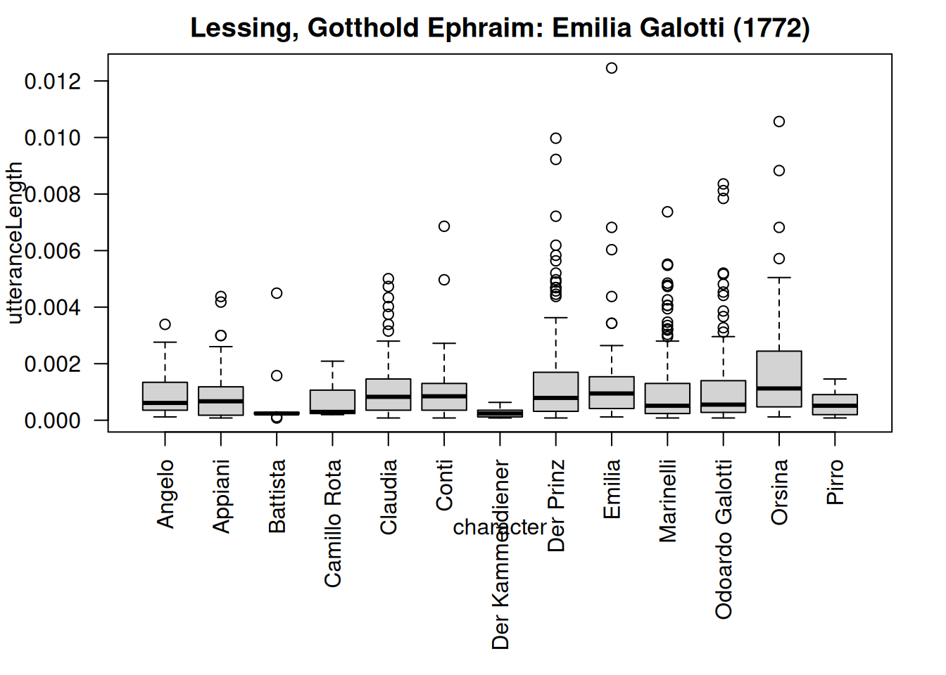
## 10   test rksp.0 der_kammerdiener           2299    3.548196e-04

This creates a table that is very long, which is why we only show the first 10 rows here. The table contains one row for each utterance, and information about the speaker of the utterance, its length (measured in tokens) and its starting position (character position). We can now inspect the variance in utterance length:

ustat <- utteranceStatistics(rksp.0) %>%
  characterNames(rksp.0)   # use names instead of character ids (see above)
  
par(mar=c(9,4,2,2)) # increase margin

boxplot(utteranceLength ~ character, # what do we want to correlate 
        data=ustat,   # the data set to use
        main = dramaNames(rksp.0), # the main title of the plot
        las = 2 # rotate axis labels
)

This uses the regular boxplot() function, enter ?boxplot for documentation. utteranceLength ~ character is called a formula in R and (in this case) expresses that we want to look at the column utteranceLength, grouped by the column character. The boxplot is a useful way to grasp the dispersion of a set of values (in this case: the lengths of all utterances by a character).

7.1 When are characters talking?

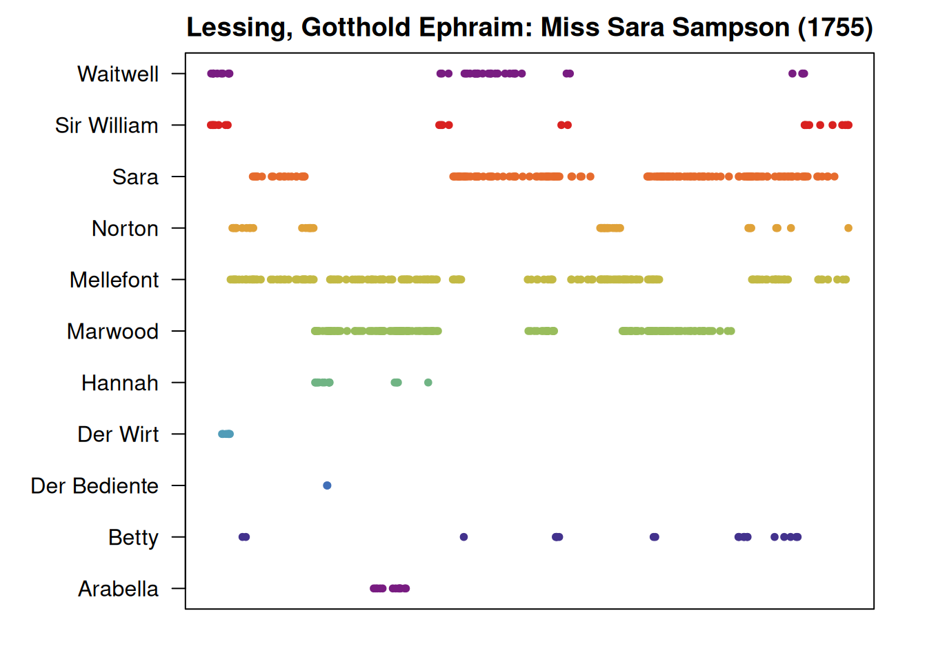
While the above displays the length of utterances, we can also display the position of utterances (remember the column utteranceBegin?). The following snippet visualizes when characters are talking, this time for Lessings Miss Sara Sampson:

par(mar=c(2,7,2,2))

utteranceStatistics(rjmw.0) %>%
  characterNames(rjmw.0) %>%    # character names instead of ids
  plot(main=dramaNames(rjmw.0))                # calling plot.QDUtteranceStatistics()

Each dot in this plot represents one utterance, the x-axis is measured in character positions. This is not really intuitive, but the flow from left to right represents the flow of the text. More technically, we again apply the function characterNames() to display character names instead of character ids. This is the same function as above, just applied to a different table. It can be applied to any table of the type QDHasCharacter. Secondly, the call to the function plot() gets rerouted to the function plot.QDUtteranceStatistics(), because the object we supply as argument is of the type QDUtteranceStatistics. Information about this function can be retrieved by entering ?plot.QDUtteranceStatistics.

7.2 Adding act boundaries

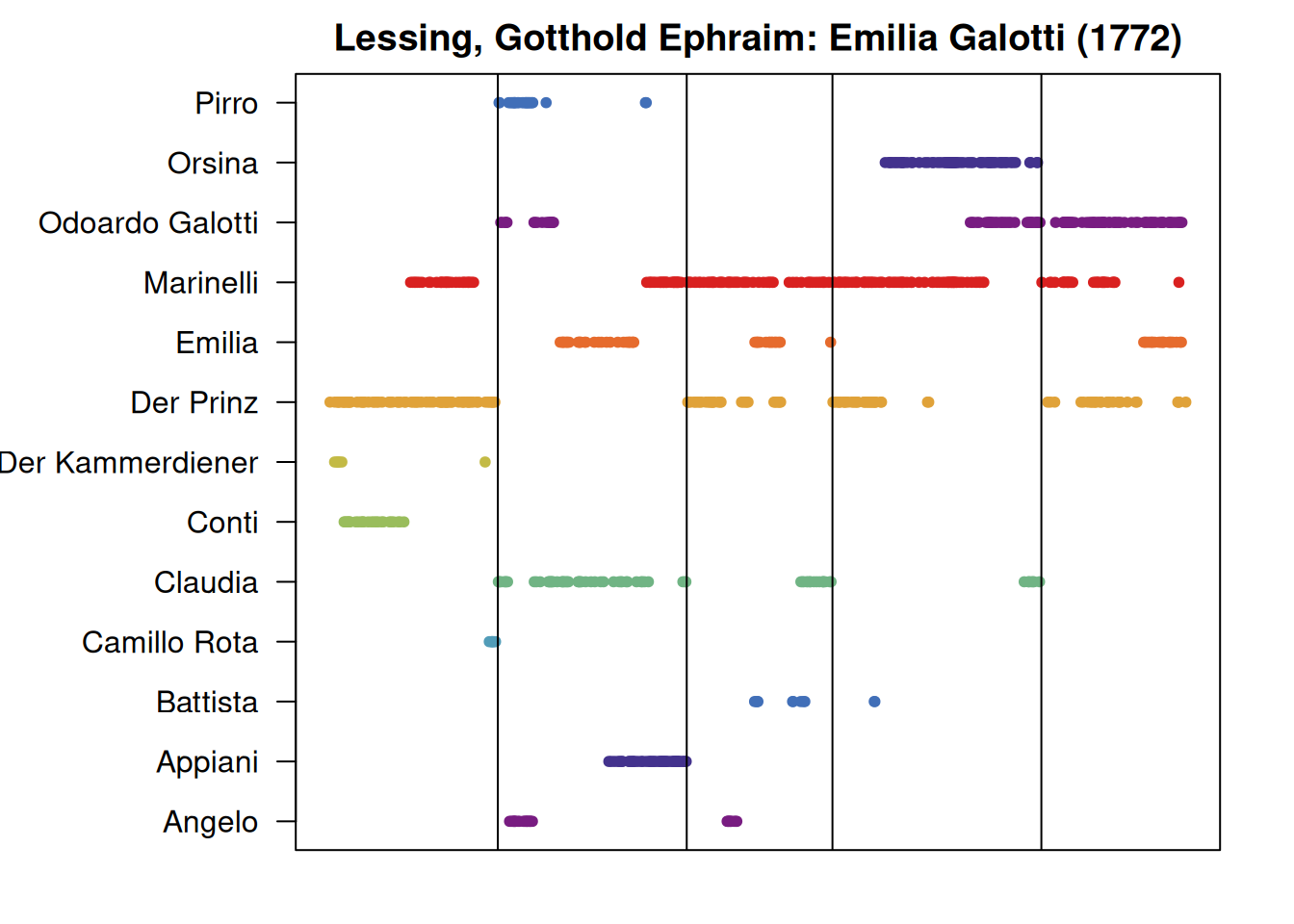
Now it would be useful to include information on act/scene boundaries in this plot. This can be done by supplying the original drama object as a second argument to the plot() function:

par(mar=c(2,8,2,2))
utteranceStatistics(rksp.0) %>%
  characterNames(rksp.0) %>%
  plot(rksp.0, # adding the `QDDrama` object here creates the act boundaries.
       main=dramaNames(rksp.0)) 

Please note that the information contained in this plot is very similar to the information in configuration matrices.

7.3 Collection analysis

In Version 3.0, the function utteranceStatistics() expects to be fed a QDDrama object that contains a single play (it will stop otherwise). It’s still possible to run it over several plays at once, if the plays are in different objects but in a single list.

We again load the Sturm und Drang plays as before, but we will use the function split() to separate the plays. This results in a list of QDDrama objects.

sturm_und_drang.ids <- c("qd:11f81.0", "qd:11g1d.0", "qd:11g9w.0", 
                         "qd:11hdv.0", "qd:nds0.0",  "qd:r12k.0", 
                         "qd:r12v.0",  "qd:r134.0",  "qd:r13g.0", 
                         "qd:rfxf.0",  "qd:rhtz.0",  "qd:rhzq.0", 
                         "qd:rj22.0",  "qd:tx4z.0",  "qd:tz39.0", 
                         "qd:tzgk.0",  "qd:v0fv.0",  "qd:wznj.0", 
                         "qd:tx4z.0",  "qd:rfxf.0")

sturm_und_drang.plays <- loadDrama(sturm_und_drang.ids)

# separate the plays
sturm_und_drang.plays <- split(sturm_und_drang.plays) 

This list can of course be plotted again, but it will result in a number of individual plots.

par(mfrow=c(length(sturm_und_drang.plays),1), mar=c(2,15,2,2))

lapply(sturm_und_drang.plays, 
       function(x) {
         utteranceStatistics(x) %>%
           characterNames(x) %>%
           plot(x, main=dramaNames(x))
       }
)