Nils Reiter
Analysing Dramatic Figure Speech with R, Part 1
This guide describes how to analyse dramatic figure speech with R, using our linguistic preprocessing tools. It is written as a step-by-step guide and uses the (German) dramatic texts Romeo und Julia and Emilia Galotti as examples.
Inhaltsverzeichnis
Before you start
This guide offers information tailored to different operating systems. Please select the appropriate one for you in the bar above.
Some basics: Both texts will be identified by their textgrid id throughout this guide and when they are loaded in the R environment. The id of Romeo und Julia isvndf.0, the id of Emilia Galotti is rksp.0.
This guide assumes that you have installed several things on your computer:
- Java
- RStudio
Please check that both are present and reasonably new.
You will also need a directory to store both downloaded code and data. Please create one now. You can name it as you like, we will use QD_DIR to refer to this directory. You will need to create several subdirectories later.
And, finally, some steps involve using a command line interface. You can launch the command line interface by searching for a program called Terminal. On Mac OS X, this is installed in /Applications/Utilities/Terminal.app. On Windows 10, it can be launched via the start menu: All Apps > Windows System > Command prompt.
Downloads
| URL | Target | Content |
|---|---|---|
| textgrid:vndf.0/data |
tei/vndf.0.xmltei\vndf.0.xml |
The TEI file containing Romeo und Julia |
| textgrid:rksp.0/data |
tei/rksp.0.xmltei\rksp.0.xml |
The TEI file containing Emilia Galotti |
| drama.Main-1.0.2.jar |
code/drama.Main.jarcode\drama.Main.jar |
Java code for doing NLP on dramatic texts |
Downloads and where to put them. All targets are relative to QD_DIR, i.e., subdirectories.
There are several things you need to download. shows the URLs. Please download the respective files into the given directories, and rename the files if necessary. Next, you need to create a directory called xmi as a subdirectory of QD_DIR.
Preprocessing
The first step will parse the TEI files, apply several NLP components to them and write the results as XMI files. XMI is an XML-based file format used to store textual data with stand-off annotations. It is used in the Apache UIMA project. While you can inspect the files, they are not made to be read by humans.
Enter the terminal, and navigate to your directory QD_DIR. Then enter the following command on a single line:
java -cp code/drama.Main.jar de.unistuttgart.ims.drama.Main.TEI2XMI --input tei --output xmi
java -cp code\drama.Main.jar de.unistuttgart.ims.drama.Main.TEI2XMI --input tei --output xmi
This should not take longer than 2 minutes, and you will see a lot of output during processing. If everything goes well, you will find the files rksp.0.xmi and vndf.0.xmi in the directory xmi (as well as a file called typesystem.xml)1.
You have now converted the TEI files into XMI, and also added a lot of linguistic and non-linguistic annotation. The next step will be exporting some of the information in the XMI files into comma-separated values-format that can be read easily with R.
Export in CSV
Again, go into the directory QD_DIR (if you have left in the meantime).
Then, execute the following command (again, enter it on a single line and press Enter on the keyboard):
java -cp code/drama.Main.jar de.unistuttgart.ims.drama.Main.XMI2UtteranceCSV --input xmi --output utterances.csv
java -cp code\drama.Main.jar de.unistuttgart.ims.drama.Main.XMI2UtteranceCSV --input xmi --output utterances.csv
You should see much less output than before. More importantly, there should be a file called utterances.csv in your QD_DIR directory. The file represents a table containing every (spoken) token in both dramatic texts along with annotations and additional information.
| drama | length | begin | end | Speaker/figure_surface | Speaker/figure_id | Token/surface | Token/pos | Token/lemma |
|---|---|---|---|---|---|---|---|---|
| vndf.0 | 29145 | 1083 | 1157 | Simson | 12 | Auf | APPR | auf |
| vndf.0 | 29145 | 1083 | 1157 | Simson | 12 | mein | PPOSAT | mein |
Header and the first two rows of utterances.csv
Utterances.csv
The following list gives a definition of each column of the file utterances.csv.
You can skip this part if you are not interested in these details.
- drama
- The drama id used in the textgrid Repository
- length
- The length of the dramatic text, measured in spoken tokens. We are not counting stage directions.
- begin
- The first character of the utterance this token (the one represented by this row) is in.
- end
- The last character of the utterance
- Speaker/figure_surface
- The name of the figure that utters this utterance. Ideally, we give the name that is introduced in the dramatic personae table at the beginning. If the name is in all upper case letters, it was not automatically mapped onto an entry in the dramatis personae table.
- Speaker/figure_id
- A numeric identifier for the figure uttering this utterance
- Token/surface
- The surface form of the token
- Token/pos
- The automatically assigned part-of-speech tag for this token, using the STTS-Tagset
- Token/lemma
- The automatically assigned lemma for this token.
Figure Speech Analysis with R
Launch R or RStudio and set the working directory to QD_DIR. Run the following commands in the R console:
# This allows us to install directly from github
install.packages("devtools")
# Load the package devtools
library(devtools)

# Install the QuaDramA R package in version 0.2.3.
# This guide has been written for 0.2.3, but if
# newer versions are available, you can try them by
# replacing the version number.
install_github("quadrama/DramaAnalysis", ref="v0.2.3")

# The steps up to here only need to be done once,
# in order to set up your installation.

# Load the package DramaAnalysis
library(DramaAnalysis)

# Now we are ready to load the dramatic texts.
# Note: this only works if you're in the right
# directory and have run the previous steps
# (successfully).
t <- read.csv("utterances.csv")
Overall Distribution
This part generates a (static) plot such as Figure 2 in this post (the stacked columns).
# We remove all figures except the 10 most
# frequently speaking
t <- limit.figures.by.rank(t)

# We calculate statistics for each figure,
# using names as identifiers
fstat <- figure.statistics(t, names=TRUE)

# we create a matrix containing the raw
# token numbers by figure rank
mat <- matrix(data=c(fstat[,3]),ncol=2)
colnames(mat) <- c(
      "Romeo und Julia (Ü: Schlegel)",
      "Emilia Galotti")
mat <- apply(mat, 2,
    function(x) {sort(x, decreasing=TRUE)})

# generate the plot
barplot(mat, beside=FALSE, col=qd.colors, border=NA, ylab = "Tokens")

# add labels to some figures
text(x=c(0.7,0.7,1.9),
    y=c(mat[1,1]/2, sum(mat[1,1]+mat[2,1]/2),
        sum(mat[1:4,2])+mat[5,2]/2),
    labels=c("Romeo", "Julia", "Emilia"),
    col=c("white"))
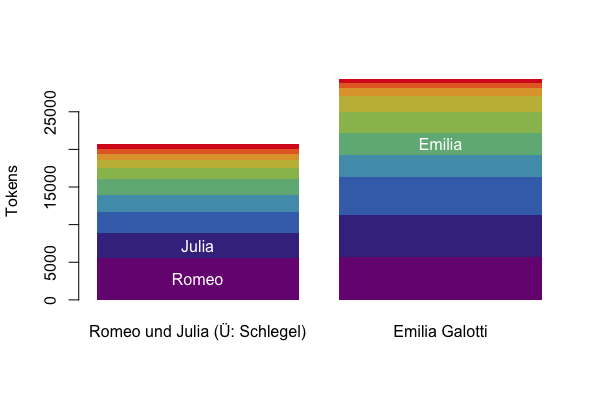
Figure Speech Distribution Plot
Variation
In this part, we generate a box plot to show the variation of utterance length.
We will restrict this analysis to the top-10 figures within one drama, vndf.0.
# make a subset of tokens to only contain vndf.0
t_vndf.0 <- t[t$drama=="vndf.0",]

# only the top 10 figures
t_vndf.0 <- limit.figures.by.rank(t_vndf.0, maxRank = 10)

# Calculate utterance statistics for all figures
ustat <- utterance_statistics(t_vndf.0, num.figures = F)

# Make a Boxplot
boxplot(ustat$utterance_length ~ ustat$figure,
          col=qd.colors, las=2, frame=F,
          main=paste("Figure Speech Variation"))
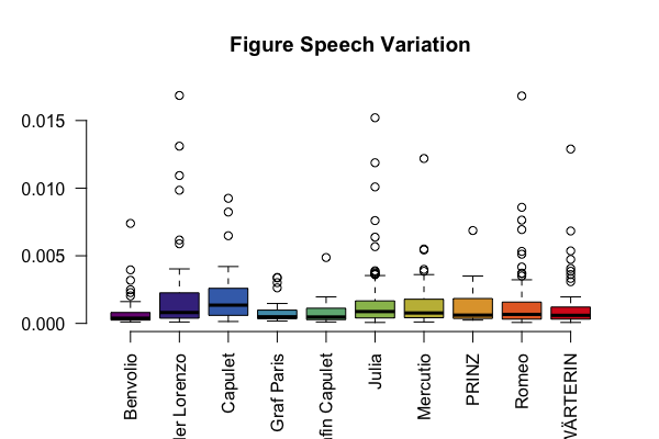
Box plot generated with R
Semantics
Now we are counting the number of words from different word fields. We are directly accessing the word lists in github.com/quadrama/metadata. The spider web plots shown in this post are displayed using Javascript in the browser, but we’ll display some other plotting options below.
# Again, we take only the top 10 figures. This makes sense for almost all analyses.
t <- limit.figures.by.rank(t, maxRank = 10)

# Count words from dictionairies by figure, normalize by figure speech
dstat <- dictionary.statistics(t, fieldnames=c("Familie", "Krieg", "Liebe", "Ratio", "Religion"), normalize = TRUE, names = TRUE)

# Order by drama, so that entries for one drama will be adjacent
dstat <- dstat[order(dstat$drama),]

# Comparing figures for a constant word field
# Make a bar graph for the word field "Familie"
# The left half of this plot are the figures in rksp.0, the right
# half are figures from vndf.0.
barplot(dstat$Familie,
  col=qd.colors, las=2,
  names.arg = dstat$figure, main="Familie")

# Comparing fields for a constant figure
# Make a bar plot showing the different fields for Romeo
barplot((unlist(dstat[dstat$figure=="Romeo",3:7])), col=qd.colors)
The resulting plots:
-

Bar plot showing amount of family words for figures in Romeo und Julia and Emilia Galotti
-
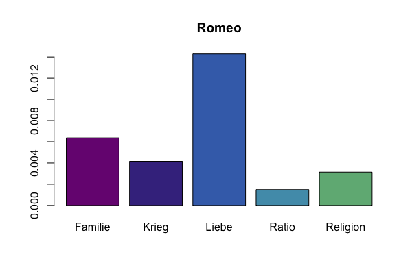
Bar plot showing different fields for Romeo
-
Added on 11.11.16: These XMI files are XML files, but they are not supposed be read by humans. Given their size (> 20MB), many XML GUI editors are not equipped to show these documents. If you want to inspect these files, you have a look at this github repository. You can download a double-clickable jar files from the releases list. ↩