Janis Pagel
Detecting Protagonists and Title Figures in Plays
In a recent paper1, we investigated how protagonists and title figures can be detected in German plays and which features are important for a machine learning model in order to conduct the classification. This post can be seen as a supplement to this paper.
Table of contents
- Basic setup
- Helper functions
- Reading in the data
- Training of a topic model
- Extraction of the features
- Prepare the data for classification
- Classification
- Evaluating the results
Basic setup
In order to run the following experiments, we need to set up some tools and prepare the data. If you want to test out the code, we provide the data that we used in our experiments. First of all, we need the data of the plays we want to analyse. We will use the GerDraCor data from https://github.com/quadrama/data_gdc. This is data in table format, extracted from a GerDraCor Fork that we created and processed using the DramaNLP Pipeline. If you would like to use your own data, you should bring it into the same format as in https://github.com/quadrama/data_gdc/tree/master/csv.
We now can load this data into R, which is the scripting language
that we will use. Basic knowledge of R is of advantage in order to
be able to follow this article more easily. For reading in the data, we will use the
DramaAnalysis package.
Install the package as given on the website. Currently this is achieved by
running the following commands:
# this is only necessary once per system
install.packages("devtools")
library(devtools)

# Install newest stable version
install_github("quadrama/DramaAnalysis", build_vignettes = TRUE)
Next, we install the GerDraCor data from the QuaDramA repositories like this:
library(DramaAnalysis)
installData(dataSource = "gdc")
installCollectionData()
This will install the data into ~/QuaDramA/Data2 by default. You can
adjust that by either issuing the setup() command or using the
dataDirectory option in installData()2. We will also use a
directory called data/ in order to store the models and other data.
You can create it anywhere ($YOUR_PATH/data) and then set up R to run commands in the
parent directory with setwd($YOUR_PATH).
We also need additional packages for the further course of this article, as listed below.
# Used libraries
library(igraph)             # For calculating centrality measures
library(data.table)         # Powerful library extending the
                            # functionality of the build-in
                            # data.frame type
library(tibble)             # Yet another data.frame implementation
library(slam)               # Sparse lightweight arrays and matrices
library(topicmodels)        # For training custom topic models
library(caret)              # Machine learning power house
library(ggplot2)            # Advanced plotting
library(iml)                # Interpretable machine learning
library(tools)              # For title case
In order to install all these package at once, issue the following command:
install.packages(c("igraph", "data.table", "tibble", "slam",
                 "topicmodels", "caret", "ggplot2", "iml",
                 "tools"))
and load them.
Helper functions
We will implement certain functions that will automate processes we will repeatedly use in the code below.
# Remove the corpus prefix from text IDs
removeCorpusPrefix <- function(str, prefix = "tg") {
  sapply(strsplit(str, paste0(prefix,":"), fixed = T),
         function(x) (if (is.na(x[2])) {x} else {x[2]}))
}

# The iml package does not make it easy to round the feature
# values for plotting. This function takes the strings of feature
# values coming from iml, transforms them into numbers, rounds them
# and returns the strings with the rounded values.
roundFeatures <- function(featureVector, n_digits = 2) {
  features <- lapply(strsplit(featureVector, "="),
                     function(x) x[1])
  values <- round(as.numeric(lapply(strsplit(featureVector, "="),
                                    function(x) x[2])),
                  digits = n_digits)
  paste0(features, "=", values)
}
Simply run this code in your R console in order to make the functions available.
Reading in the data
We read in the data using DramaAnalysis functions. We will want to
analyse the plays regarding their genre. To this end, we use predefined categorizations
and load them via loadSet() (the lists
already got installed above using installCollectionData()). Then we
load the texts for the categorized plays3. Since the loading of the
texts takes some time, we store the data on disk. This way, we can
simply reload the texts in a new session.
# Load text IDs based on their genre
ids.corpora <- list(sd=as.character(loadSet("sturm_und_drang")),
                    bt=as.character(loadSet(
                                  "buergerliches_trauerspiel")),
                    wk=as.character(loadSet("weimarer_klassik")),
                    pop=as.character(loadSet("populaere_stuecke")),
                    nat=as.character(loadSet("naturalismus")),
                    wm=as.character(loadSet("wiener_moderne")),
                    rom=as.character(loadSet("romantik")),
                    auf=as.character(loadSet("aufklaerung")),
                    vm=as.character(loadSet("vormaerz"))
                    )
ids.corpora <- lapply(ids.corpora,
               function(x) (gsub("tg", "gdc", x, fixed = TRUE)))
ids.all <- unique(Reduce(c, ids.corpora))
ids.all <- removeCorpusPrefix(ids.all, prefix = "gdc")

# Load the texts
texts <- loadSegmentedText(ids.all, defaultCollection = "gdc")
# Remove rows with unknown speakers
texts <- texts[!is.na(texts$Speaker.figure_surface)]
# Save texts for later use
save(texts, file="data/texts.RData")
In the above mentioned paper, we investigated both detecting
protagonists and title figures. From a technical point of view, the
classification of figures into protagonists or title figures follows
the same steps. We further proceed with using annotations that name
figures which are title figures, but you could as well replace it with
an annotation of protagonists or any other binary class of figures that might
be classified by the used features. We read in the annotations from a
file called titlefigures.csv.
Download it from here
and save it under $YOUR_PATH/data/titlefigures.csv.
The format of that file follows the structure
Drama1,Titlefigure1,
Drama2,Titlefigure2,Titlefigure3
Drama3,Titlefigure4,
...
...
...
i.e. the first column contains the drama ID, and all following columns contain the ID of the title figure(s), depending on the number of title figures for that play. In our data, there were never more than two title figures for a play, but you might want to extend or reduce the number of columns depending on your own data. Just make sure that the number of commas for each row matches up to the maximal number of columns. Given this kind of file, reading in the information is easy:
heroes <- data.table(read.csv("data/titlefigures.csv",
                              header = FALSE))
heroes <- melt(heroes, id.vars = "V1", na.rm = TRUE)
heroes$variable <- NULL
heroes <- heroes[value!="",]
colnames(heroes) <- c("drama", "figure")
We additionally coerce the data table into a format that lists each title figure on a separate row, together with the respective drama ID, and rename the columns for more verbosity.
Training of a topic model
We noticed that training a topic model on the data we wanted to classify let to slightly better results than using a pre-trained model on prose text. We accomplish this as follows:
ldaModels <- list()
ft <- as.simple_triplet_matrix(as.matrix(frequencytable(texts,
                               normalize = FALSE)))
ldaModels$lda_5 <- LDA(ft, k = 5, method = "Gibbs")
ldaModels$lda_10 <- LDA(ft, k = 10, method = "Gibbs")
save(ldaModels, file = "data/ldaModels.RData")
The texts variable contains the texts we want to train the topic
model on and which we already read in in the section above. We use the
frequencytable() function from the DramaAnalysis package in order to
create a frequency table containing word frequencies per drama and store it in ft. We then train
the topic models using the topicmodels package. You can experiment
with different models; we opted to use Latent Dirichlet Allocation in combination with
Gibbs sampling and train two models with 5 and 10 clusters
respectively. We then store the models for later use.
Extraction of the features
It is time to extract all features we want to use to later train a machine learning model. To that end, we load the previously loaded texts and the topic model we wish to use. Furthermore, we extract all IDs of the dramas we have annotations for. This way, we reduce the data size and do not compute features for unnecessary texts.
# Load the texts in case they are not in memory anymore
load("data/texts.RData")
# Load the topic models
load("data/ldaModels.RData")

ids <- ids.all[ids.all %in% unique(heroes$drama)]
We then iterate over all texts and store all figures of each play into a
giant data.table, called p. This data.table contains a list of all figures per
row and stores their ID, as well as the ID of the respective drama in
its columns. Additional columns store any kind of feature we wish to
use. In our case, this will be:
- Number of figures for a play
- Degree Centrality
- Weighted Degree Centrality
- Betweenness Centrality
- Closeness Centrality
- Eigenvector Centrality
- Posterior probability for each cluster of the topic model
- Presence in the last act
- Number of active scenes
- Number of passive scenes
- Number of uttered tokens
- Affiliation of a drama to a specific genre
There are also other types of information, such as the number of
utterances a figure makes or the token ID of when the figure speaks
firstly and lastly.
This information comes from functions located in the DramaAnalysis
package and gets automatically
merged into the final data.table. We will not use this information in
the following experiments, but some of it might be useful for future
experiments and, of course, additional features can be added freely.
Now, have a look at the concrete code:
p <- Reduce(rbind, lapply(ids, function(x) {
  # Get a single text
  text <- texts[drama==x]
  # Create a table with the characters
  char <- unique(texts[which(texts$drama==x),
                       c("corpus",
                         "drama",
                         "Speaker.figure_surface",
                         "Speaker.figure_id")])
  # Get the overall number of characters
  nfig <- nrow(char)
  # Create a presence matrix
  pres <- presence(text, passiveOnlyWhenNotActive = TRUE)
  # Get the number of tokens a character utters
  fstat <- figureStatistics(text)
  ft <- frequencytable(text, names = FALSE,
                       column = "Token.lemma", normalize = FALSE,
                       byFigure = TRUE)
  # Create a co-presence matrix
  conf <- configuration(text,by="Scene",onlyPresence = TRUE,
                        useCharacterId = TRUE)
  copr <- conf$matrix %*% t(conf$matrix)
  rownames(copr) <- conf$figure
  colnames(copr) <- conf$figure
  # Find out if a character appeared in the last act
  confAct <- configuration(text, by="Act", onlyPresence = TRUE,
                           useCharacterId = TRUE)
  lastAct <- cbind(confAct$drama, figure = confAct$figure,
                   lastAct = as.numeric(confAct$matrix[,
                                        ncol(confAct$matrix)]))
  # Get a co-presence graph based on the co-presence matrix
  g <- graph_from_adjacency_matrix(copr, mode = "upper",
                                   diag = FALSE, weighted = TRUE)
  # Calculate different centrality measures
  dg <- degree(g, normalized = TRUE)
  wdg <- strength(g)
  bt <- betweenness(g, normalized = TRUE)
  cn <- closeness(g, normalized = TRUE)
  ev <- eigen_centrality(g)
  # Get the posterior probability for a character to be part
  # of a certain topic, based on their uttered tokens
  post <- posterior(ldaModels$lda_10, ft)$topics
  post.df <- data.frame(figure = substr(rownames(post),
                                        8,
                                        100),
                        post)
  # Merge all features into a feature table with each character
  # as a row
  pres <- merge(pres, char,
                by.x = c("corpus", "drama", "figure"),
                by.y = c("corpus", "drama", "Speaker.figure_id"))
  pres$nfig <- rep(nfig, nrow(pres))
  pres <- merge(pres, lastAct)
  pres <- merge(pres, fstat)
  pres <- merge(pres, post.df, by = c("figure"))
  pres <- merge(pres, data.frame(degree = dg, figure = names(dg)))
  pres <- merge(pres, data.frame(wdegree = wdg,
                                 figure = names(wdg)))
  pres <- merge(pres, data.frame(between = bt, figure = names(bt)))
  pres <- merge(pres, data.frame(close = cn, figure = names(cn)))
  pres <- merge(pres, data.frame(eigen = ev$vector,
                                 figure = names(ev$vector)))
  # Return the feature table
  pres
}))
After p got created, we make some adjustments. The drama column
should be converted into factors. For better readability, we also
rename the columns which got automatically created by the topic model
and replace the generated X with T (for topic). The information
about
which drama belongs into which genre is independent of the figure and
can be added now. Lastly, we need to determine, wether a figure was
actually a title figure or not, based on our annotations. To achieve
this, we
use the previously created heroes data.table and store the classes
into a column class. If the figure belongs to the title figure class,
we store TF (title figure), otherwise NTF (not title figure).
The labels are arbitrary though. Optionally, we might
also want to store the data.frame for later use.
p$drama <- factor(p$drama)
names(p) <- gsub("X", "T", names(p), fixed = TRUE)

p$SD <- as.integer(paste(p$corpus, p$drama, sep = ":")
                   %in% ids.corpora$sd)
p$BT <- as.integer(paste(p$corpus, p$drama, sep = ":")
                   %in% ids.corpora$bt)
p$WK <- as.integer(paste(p$corpus, p$drama, sep = ":")
                   %in% ids.corpora$wk)
p$POP <- as.integer(paste(p$corpus, p$drama, sep = ":")
                   %in% ids.corpora$pop)
p$NAT <- as.integer(paste(p$corpus, p$drama, sep = ":")
                   %in% ids.corpora$nat)
p$WM <- as.integer(paste(p$corpus, p$drama, sep = ":")
                   %in% ids.corpora$wm)
p$ROM <- as.integer(paste(p$corpus, p$drama, sep = ":")
                   %in% ids.corpora$rom)
p$AUF <- as.integer(paste(p$corpus, p$drama, sep = ":")
                   %in% ids.corpora$auf)
p$VM <- as.integer(paste(p$corpus, p$drama, sep = ":")
                   %in% ids.corpora$vm)

p$class <- ifelse(apply(p, 1, function(x) (if (any(x["drama"] ==
                    heroes$drama & x["figure"] == heroes$figure))
                    {TRUE} else {FALSE})),
                  "TF",
                  "NTF")
p$class <- factor(p$class)

save(p, file = "data/p.RData")
> head(p)

      figure corpus  drama scenes actives passives
1:   andreas    gdc tzgk.0     75       5       13
2:  arabella    gdc tzgk.0     75       5        2
3:  asserato    gdc tzgk.0     75       3        2
4: bedienter    gdc tzgk.0     75       1        2
5:     bella    gdc tzgk.0     75       2        8
6:     berta    gdc tzgk.0     75       4        6
      presence Speaker.figure_surface nfig lastAct
1: -0.10666667                ANDREAS   38       1
2:  0.04000000               ARABELLA   38       1
3:  0.01333333               ASSERATO   38       0
4: -0.01333333              BEDIENTER   38       0
5: -0.08000000                  BELLA   38       0
6: -0.02666667                  BERTA   38       1
   length tokens types utterances utteranceLengthMean
1:  32469    820   406         25           32.800000
2:  32469    288   160         21           13.714286
3:  32469    149   100         15            9.933333
4:  32469     10    10          1           10.000000
5:  32469    104    81          3           34.666667
6:  32469    212   111         32            6.625000
   utteranceLengthSd firstBegin lastEnd         T1
1:         25.734218      77418  196198 0.03171953
2:         12.810710       3603  189928 0.06400000
3:          4.511361      62813  144980 0.04697987
4:                NA     152575  152646 0.12500000
5:         32.129944      75759  154735 0.07500000
6:          3.687380      35983  197145 0.16756757
           T2         T3         T4        T5
1: 0.04006678 0.02838063 0.03672788 0.2520868
2: 0.03200000 0.03600000 0.06800000 0.0760000
3: 0.04026846 0.04026846 0.05369128 0.2080537
4: 0.08928571 0.08928571 0.08928571 0.1071429
5: 0.05833333 0.05833333 0.06666667 0.3250000
6: 0.05405405 0.04864865 0.05405405 0.1621622
           T6        T7         T8         T9
1: 0.01001669 0.5292154 0.02337229 0.02671119
2: 0.02400000 0.5680000 0.03600000 0.04400000
3: 0.03355705 0.4362416 0.04697987 0.04697987
4: 0.08928571 0.1428571 0.08928571 0.08928571
5: 0.05000000 0.2083333 0.05833333 0.05000000
6: 0.05945946 0.3027027 0.06486486 0.04864865
          T10     degree wdegree      between
1: 0.02170284 0.16216216       8 0.0193078793
2: 0.05200000 0.21621622      11 0.1005694872
3: 0.04697987 0.24324324      15 0.0516348166
4: 0.08928571 0.02702703       1 0.0000000000
5: 0.05000000 0.05405405       4 0.0000000000
6: 0.03783784 0.10810811       7 0.0005744381
       close       eigen SD BT WK POP NAT WM ROM AUF
1: 0.4512195 0.069323313  1  0  0   0   0  0   0   0
2: 0.4868421 0.105234584  1  0  0   0   0  0   0   0
3: 0.4252874 0.251059554  1  0  0   0   0  0   0   0
4: 0.3557692 0.026868517  1  0  0   0   0  0   0   0
5: 0.2242424 0.008853292  1  0  0   0   0  0   0   0
6: 0.3814433 0.164283361  1  0  0   0   0  0   0   0
   VM class
1:  0   NTF
2:  0   NTF
3:  0   NTF
4:  0   NTF
5:  0   NTF
6:  0   NTF
Prepare the data for classification
We now make some last adjustments before training a model on the
extracted features. We normalise the actives, passives and tokens
features by the overall length of the play. For plotting purposes, we
also bring the character surface string into a nice title case format.
We then backup this original table and remove all information that the
machine learning should not have any access to. We save both the
original dataset and the training dataset into the variable pTF.
prepareData <- function(p) {
  p[is.na(p)] <- 0
  p <- na.omit(p)

  p$actives <- p$actives/p$scenes
  p$passives <- p$passives/p$scenes
  p$tokens <- p$tokens/p$length
  p$presence <- NULL
  p$Speaker.figure_surface <- toTitleCase(tolower(
                                        as.character(
                                        p$Speaker.figure_surface)))
  orig <- p
  p$corpus <- NULL
  p$figure <- NULL
  p$length <- NULL
  p$scenes <- NULL
  p$Speaker.figure_surface <- NULL
  p$drama <- as.integer(p$drama)
  list(p = p, orig = orig)
}

pTF <- prepareData(p)
Classification
First, we define the machine learning method we want to use. We will use
a random forest classifier in conjunction with the
caret package, but other
classifiers are also viable. The function testFeatureSet() is a
convenience method. It allows us to make sure that every time we call a
caret classification, the same seed will be set. We can also give in
the sampling method we wish to use. Furthermore, we can
experiment with different sets of features. The output of that function
is a list containing the trained model, the input and output data of
that model, the feature importance specific to the model, a confusion
matrix of the result, the concrete prediction as well as the correct
and the incorrect predictions for later error analysis. We can also
already define different combinations of features we wish to try out.
The feature names are simply the column names of pTF.
# Define which classifier to use
caretMethod <- "rf"
# Define the number of sampling repeats
repeatsVariable <- 10
# Set seed for the random number generator
seed <- 42
set.seed(seed)

testFeatureSet <- function(features, p, orig, sampling, seed = 42) {
  set.seed(seed)
  fv <- as.matrix(subset(p, select = -c(class)))
  x <- fv[, features, drop = FALSE]
  x <- as.data.frame(x)
  control <- trainControl(method = "repeatedcv",
                          number = 10,
                          repeats = repeatsVariable,
                          savePredictions = "all",
                          sampling = sampling,
                          classProbs = TRUE)
  model <- train(x = x,
                 y = p$class,
                 method = caretMethod,
                 trControl = control,
                 preProc = c("center", "scale"))
  if (length(features) > 1) {
    varI <- varImp(model, scale = FALSE)
  } else {
    varI <- data.frame()
  }
  predictions <- predict(model, x)
  cm  <- list(TF = confusionMatrix(predictions,
                                  p$class,
                                  mode = "everything",
                                  positive = "TF"),
              NTF = confusionMatrix(predictions,
                                  p$class,
                                  mode = "everything",
                                  positive = "NTF"))
  pred <- data.frame(orig[,c("corpus", "drama", "figure", "BT",
                             "WK", "SD", "POP", "NAT",
                             "WM", "ROM", "AUF", "VM")],
                     pred = predictions, ref = orig[, "class"])
  falsePredictions <- pred[pred$pred != pred$class, ]
  correctPredictions <- pred[pred$pred == pred$class, ]
  list(model = model, x = x, y = p$class, imp = varI, cm = cm,
       pred = pred, correct = correctPredictions,
       mistakes = falsePredictions)
}

features <- c(c("BT" ,"WK", "SD", "POP", "NAT", "WM", "ROM",
                "AUF", "VM"),
              "tokens",
              c("degree", "wdegree", "close", "eigen", "between"),
              c("actives", "passives"),
              paste0("T",1:10),
              "nfig",
              "lastAct")
featuresWithoutTokens <- c(c("BT" ,"WK", "SD", "POP", "NAT",
                             "WM", "ROM", "AUF", "VM"),
                           c("degree", "wdegree", "close",
                             "eigen", "between"),
                           c("actives", "passives"),
                           paste0("T",1:10),
                           "nfig",
                           "lastAct")
We now simply call testFeatureSet() with different features and the
desired sampling method. For example, as a simple baseline,
we could only use the tokens feature.
We also train two models, one with all features and one with all features minus the
tokens feature, respectively. As the sampling method, we make use of
smote. Afterwards, we save the models on disk for later use and
evaluation.
results <- list()

results$TokensBL <- testFeatureSet("tokens",
                                   pTF$p,
                                   pTF$orig,
                                   sampling = "smote",
                                   seed)
results$woTokens <- testFeatureSet(featuresWithoutTokens,
                                   pTF$p,
                                   pTF$orig,
                                   sampling = "smote",
                                   seed)
results$All <- testFeatureSet(features,
                              pTF$p,
                              pTF$orig,
                              sampling = "smote",
                              seed)

save(results, file = "data/results.RData")
Evaluating the results
We can now evaluate the models in different ways4:
- Confusion matrix of predicted classes against actual classes of characters
- Feature importance
- Prediction for single characters
Let us start with confusion matrices. We can retrieve the confusion
matrix for a model and a specific class from the outputted list of testFeatureSet():
cm <- results$All$cm$TF$table
> cm

          Reference
Prediction  NTF   TF
       NTF 1100    0
       TF    66   42
Next, we might also want to calculate different evaluation metrics based on the confusion matrix, such as precision, recall, F1 and accuracy. This can also easily be done for all models at once to make a comparison:
dfTF <- data.frame(lapply(results, function(x) {x$cm$TF$byClass}))
dfNTF <- data.frame(lapply(results, function(x) {x$cm$NTF$byClass}))
dfO <- data.frame(lapply(results, function(x) {x$cm$NTF$overall}))

dfEval <- rbind(dfTF, dfNTF, dfO)
dfEval <- dfEval[c("Precision", "Recall", "F1", "Accuracy"),]
> dfEval

           TokensBL  woTokens       All
Precision 0.3387097 0.3281250 0.3888889
Recall    1.0000000 1.0000000 1.0000000
F1        0.5060241 0.4941176 0.5600000
Accuracy  0.9321192 0.9288079 0.9453642
We can retrieve and plot the feature importance in the following way:
imp <- results$All$imp$importance %>%
  as.data.frame() %>%
  rownames_to_column() %>%
  ggplot(aes(x = reorder(rowname, Overall), y = Overall)) +
    geom_bar(stat = "identity", alpha = 0.8) +
    coord_flip() +
    labs(x = "Feature", y = "Importance")
> imp
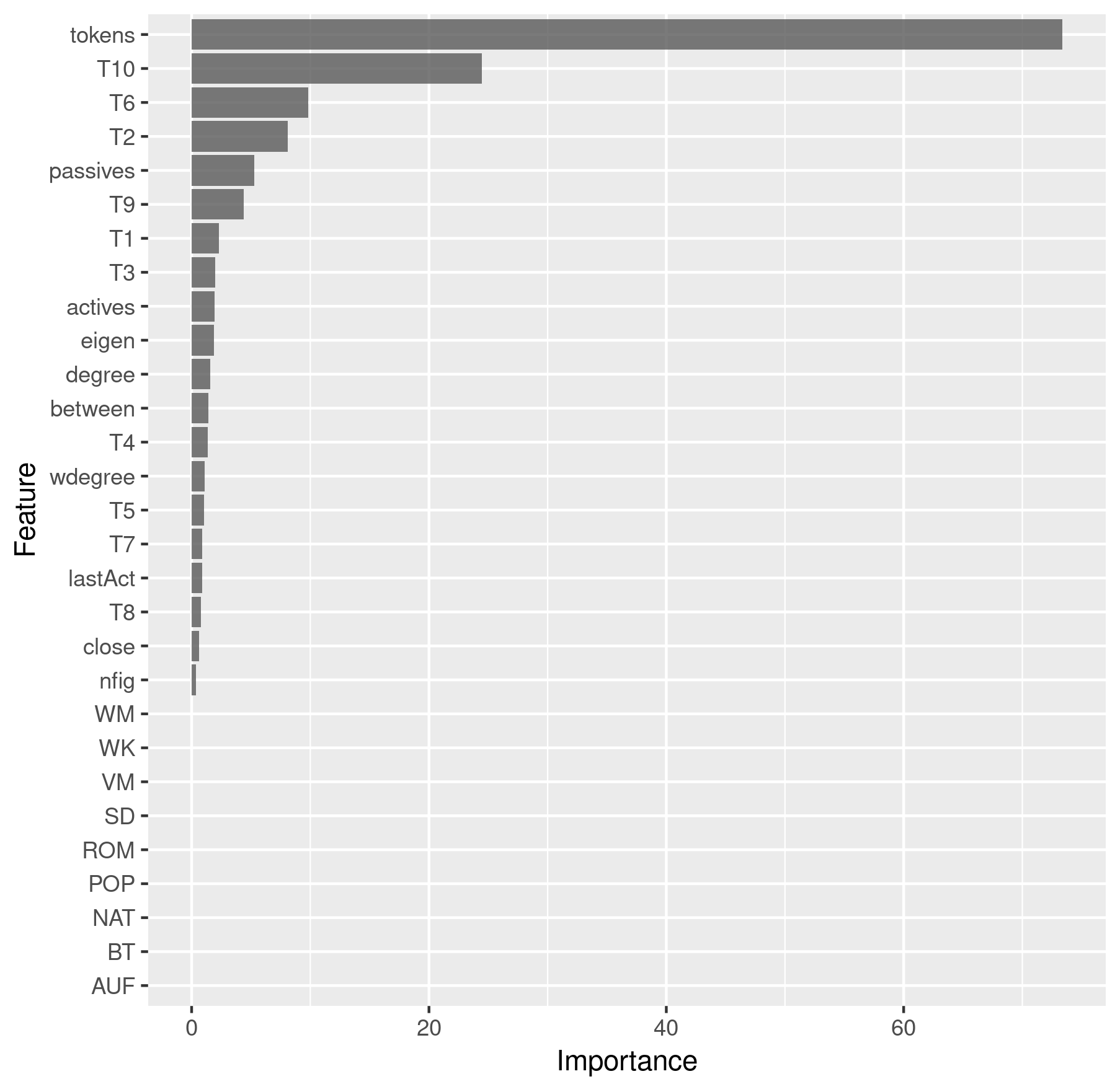
Feature importance
Lastly, we can also inspect the model’s prediction for a single character. This can be interesting if we suspect a character to be especially difficult to classify and we can also inspect the predictions for multiple characters and compare them. Let’s take Emilia and Marinelli from Lessing’s Emilia Galotti as examples. Of course, we are interested in knowing if the model managed to predict them correctly.
chars <- c("emilia", "marinelli")
predChar <- results$All$pred[results$All$pred$figure %in% chars &
                results$All$pred$drama == "rksp.0", ][,
                c("corpus", "drama", "figure", "class", "pred")]
> predChar

corpus  drama    figure class pred
   gdc rksp.0    emilia    TF   TF
   gdc rksp.0 marinelli   NTF   TF
We see that Emilia was predicted correctly as a title figure, but the model assumed that Marinelli would be a title figure as well, which is incorrect.
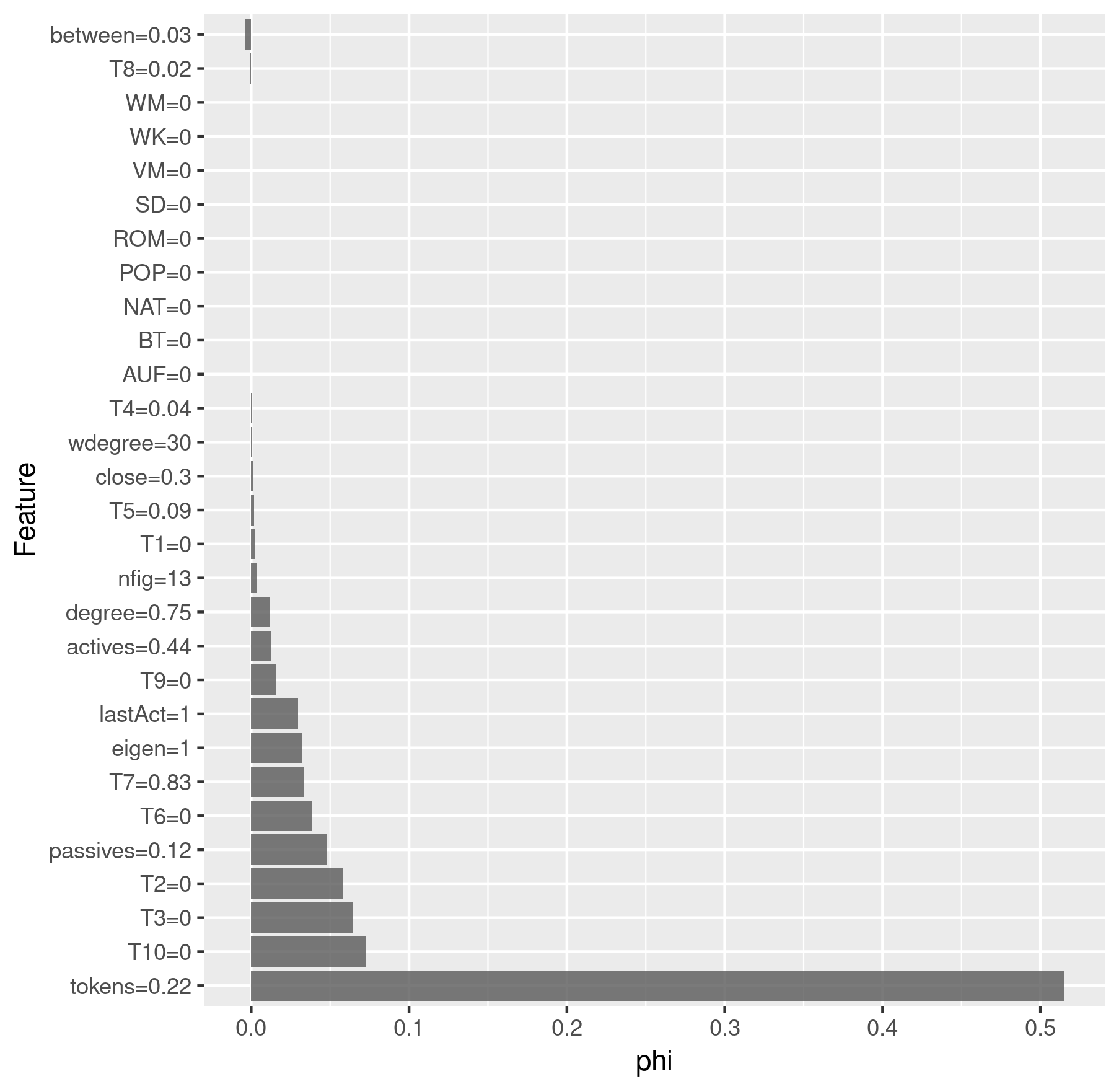
Finally, we apply a Shapley analysis which shows the importance of the
features for the classification of a single data point. The higher the
value phi, the more important the feature was. A negative phi
indicates that the feature was contra-productive to assign the character
to the class. We use the iml
package to perform the Shapley analysis. First we need to create an
iml predictor:
x <- results$All$x
y <- results$All$y
predictor <- Predictor$new(results$All$model, data = x, y = y)
Then we can compute the Shapley values for a single character and plot the results:
charID <- rownames(results$All$pred[
                   results$All$pred$figure == "emilia"
                   & results$All$pred$drama == "rksp.0", ])
shapley <- Shapley$new(predictor, x.interest = x[charID, ])
# Round the feature values so that they don't clutter the plot
shapley$results$feature.value <-
                    roundFeatures(shapley$results$feature.value)
shapley_emilia <- shapley$results[
                  which(shapley$results$class == "TF"), ] %>%
  ggplot(aes(x = reorder(feature.value, -phi), y = phi)) +
    geom_bar(stat = "identity", alpha = 0.8) +
    coord_flip() +
    labs(x = "Feature", y = "phi")

charID <- rownames(results$All$pred[
                   results$All$pred$figure == "marinelli"
                   & results$All$pred$drama == "rksp.0", ])
shapley$explain(x.interest = x[charID, ])
shapley$results$feature.value <-
                    roundFeatures(shapley$results$feature.value)
shapley_marinelli <- shapley$results[
                     which(shapley$results$class == "TF"), ] %>%
  ggplot(aes(x = reorder(feature.value, -phi), y = phi)) +
    geom_bar(stat = "identity", alpha = 0.8) +
    coord_flip() +
    labs(x = "Feature", y = "phi")
> shapley_emilia

Shapley analysis for Emilia
> shapley_marinelli
Shapley analysis for Marinelli
That’s all for now. You get the complete running code from here.
-
The paper is orginally written in German and got translated into English by the publisher. ↩
-
For a more thorough and up-to-date description, see the DramaAnalysis Wiki. ↩
-
As the collections are currently only available for TextGrid, some texts will not be loaded, since they are not available in GerDraCor. Any error message in R about this can be ignored safely. ↩
-
The implementation of point 2 and 3 was heavily inspired by https://www.r-bloggers.com/interpretable-machine-learning-with-iml-and-mlr/ and https://shirinsplayground.netlify.com/2018/07/explaining_ml_models_code_caret_iml/. Check out their content for more ideas on interpreting blackbox models using R. ↩